slendr simulations

practical workshop at MPI EVA Leipzig

Author

Martin Petr

Published

February 2023

Many problems in population genetics cannot be solved by a mathematician, no matter how gifted. [It] is already clear that computer methods are very powerful. This is good. It […] permits people with limited mathematical knowledge to work on important problems […]

James F. Crow – interview

Why use simulations?

Making sense of estimated statistics
Fitting model parameters
Ground truth for method work

Making sense of estimated statistics

Hajdinjak (2021)

Making sense of estimated statistics

Palkopoulou (2018)

Making sense of estimated statistics

Petr (2019)

Fitting model parameters (i.e. ABC)

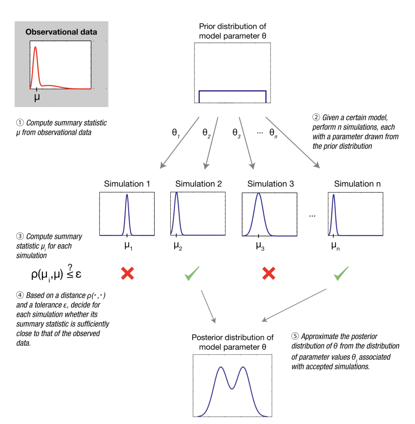
Image from Wikipedia on ABC

Ground truth for methods work

Schiffels and Durbin (2014)

There are many simulation tools

The most famous and widely used are SLiM and msprime.

Both are very powerful…

… but they require a lot of programming knowledge...

… and a lot of code for non-trivial simulations (🐛🪲🐜).

This is why we will focus on slendr,
a convenient R interface to both SLiM and msprime.

SLiM

What is SLiM?

Forward-time simulator

It’s fully programmable!

Massive library of functions for:
- Demographic events
- Various mating systems
- Selection, quantitative traits, …

> 700 pages long manual!

SLiMgui – IDE for SLiM

Simple neutral simulation in SLiM

initialize() {
    // create a neutral mutation type
    initializeMutationType("m1", 0.5, "f", 0.0);
    // initialize 1Mb segment
    initializeGenomicElementType("g1", m1, 1.0);
    initializeGenomicElement(g1, 0, 999999);
    // set mutation rate and recombination rate of the segment
    initializeMutationRate(1e-8);
    initializeRecombinationRate(1e-8);
}

// create an ancestral population p1 of 10000 diploid individuals
1 early() { sim.addSubpop("p1", 10000); }

// in generation 1000, create two daughter populations p2 and p3
1000 early() {
    sim.addSubpopSplit("p2", 5000, p1);
    sim.addSubpopSplit("p3", 1000, p1);
}

// in generation 10000, stop the simulation and save 100 individuals
// from p2 and p3 to a VCF file
10000 late() {
    p2_subset = sample(p2.individuals, 100);
    p3_subset = sample(p3.individuals, 100);
    c(p2_subset, p3_subset).genomes.outputVCF("/tmp/slim_output.vcf.gz");
    sim.simulationFinished();
    catn("DONE!");
}

msprime

What is msprime?

A Python module for writing coalescent simulations

Extremely fast (genome-scale, population-scale data)

You must know Python fairly well to build complex models

Simple simulation using msprime

This is basically the same model as the SLiM script earlier:

import msprime

demography = msprime.Demography()
demography.add_population(name="A", initial_size=10_000)
demography.add_population(name="B", initial_size=5_000)
demography.add_population(name="C", initial_size=1_000)
demography.add_population_split(time=1000, derived=["A", "B"], ancestral="C")

ts = msprime.sim_ancestry(
  sequence_length=10e6,
  recombination_rate=1e-8,
  samples={"A": 100, "B": 100},
  demography=demography
)

source: link

www.slendr.net

Why a new package? – spatial simulations!

Why a new package?

Most researchers are not expert programmers
All but the most trivial simulations require lots of code

90% of simulations are basically the same!
- create populations (splits and \(N_e\) changes)
- specify if/how they should mix (rates and times)
- save output (VCF, EIGENSTRAT)

Lot of code duplication across projects

Let’s get started

We will need slendr & tidyverse

# load data analysis and plotting packages
library(dplyr)


Attaching package: 'dplyr'

The following objects are masked from 'package:stats':

    filter, lag

The following objects are masked from 'package:base':

    intersect, setdiff, setequal, union

library(ggplot2)
library(magrittr)

# load slendr itself
library(slendr)

=======================================================================
NOTE: Due to Python setup issues on some systems which have been
causing trouble particularly for novice users, calling library(slendr)
no longer activates slendr's Python environment automatically.

In order to use slendr's msprime back end or its tree-sequence
functionality, users must now activate slendr's Python environment
manually by executing init_env() after calling library(slendr).

(This note will be removed in the next major version of slendr.)
=======================================================================


Attaching package: 'slendr'

The following object is masked from 'package:magrittr':

    subtract

init_env()

The interface to all required Python modules has been activated.

(ignore the message about missing SLiM)

slendr haiku

Build simple models,

simulate data from them.

Just one plain R script.

Typical steps (outline of this tutorial)

creating populations
scheduling population splits
programming \(N_e\) size changes
encoding gene-flow events
simulation sequence of a given size
computing statistics from simulated outputs

Creating a `population()`

Each needs a name, size and time of appearance (i.e., “split”):

pop1 <- population("pop1", N = 1000, time = 1)

This creates a normal R object. Typing it gives a summary:

pop1

slendr 'population' object 
-------------------------- 
name: pop1 
non-spatial population
stays until the end of the simulation

population history overview:
  - time 1: created as an ancestral population (N = 1000)

Programming population splits

Splits are indicated by the parent = <pop> argument:

pop2 <- population("pop2", N = 100, time = 50, parent = pop1)

The split is reported in the “historical summary”:

pop2

slendr 'population' object 
-------------------------- 
name: pop2 
non-spatial population
stays until the end of the simulation

population history overview:
  - time 50: split from pop1 (N = 100)

Scheduling resize events – `resize()`

Step size decrease:

pop1 <- population("pop1", N = 1000, time = 1)
pop1_step <- resize(pop1, N = 100, time = 500, how = "step")

Exponential increase:

pop2 <- population("pop2", N = 100, time = 50, parent = pop1)
pop2_exp <- resize(pop2, N = 10000, time = 500, end = 2000, how = "exponential")

Tidyverse-style pipe `%>%` interface

A more concise way to express the same thing as before.

Step size decrease:

pop1 <-
  population("pop1", N = 1000, time = 1) %>%
  resize(N = 100, time = 500, how = "step")

Exponential increase:

pop2 <-
  population("pop2", N = 1000, time = 1) %>%
  resize(N = 10000, time = 500, end = 2000, how = "exponential")

A more complex model

pop1 <- population("pop1", N = 1000, time = 1)

pop2 <-
  population("pop2", N = 1000, time = 300, parent = pop1) %>%
  resize(N = 100, how = "step", time = 1000)

pop3 <-
  population("pop3", N = 1000, time = 400, parent = pop2) %>%
  resize(N = 2500, how = "step", time = 800)

pop4 <-
  population("pop4", N = 1500, time = 500, parent = pop3) %>%
  resize(N = 700, how = "exponential", time = 1200, end = 2000)

pop5 <-
  population("pop5", N = 100, time = 600, parent = pop4) %>%
  resize(N = 50, how = "step", time = 900) %>%
  resize(N = 250, how = "step", time = 1200) %>%
  resize(N = 1000, how = "exponential", time = 1600, end = 2200) %>%
  resize(N = 400, how = "step", time = 2400)

Remember that slendr objects internally carry their whole history!

pop5

slendr 'population' object 
-------------------------- 
name: pop5 
non-spatial population
stays until the end of the simulation

population history overview:
  - time 600: split from pop4 (N = 100)
  - time 900: resize from 100 to 50 individuals
  - time 1200: resize from 50 to 250 individuals
  - time 1600-2200: exponential resize from 250 to 1000 individuals
  - time 2400: resize from 1000 to 400 individuals

Last step before simulation: `compile_model()`

model <- compile_model(
  list(pop1, pop2, pop3, pop4, pop5),
  generation_time = 1,
  simulation_length = 3000
)

Compilation takes a list of model components, performs internal consistency checks, returns a single model object.

The model is also compiled to disk which gives a nice additional layer of reproducibility. The exact location can be specified via path = argument to compile_model().

Model summary

Typing the compiled model into R prints a brief summary:

model

slendr 'model' object 
--------------------- 
populations: pop1, pop2, pop3, pop4, pop5 
geneflow events: [no geneflow]
generation time: 1 
time direction: forward 
total running length: 3000 model time units
model type: non-spatial

configuration files in: /private/var/folders/d_/hblb15pd3b94rg0v35920wd80000gn/T/Rtmp8Mdden/filed642a032e2

Model visualization

plot_model(model)

Exercise #1

Exercise #1 — write your own model!

You can use this “template”:

library(slendr)
init_env()

chimp <- population(...)
# <... rest of your code ...>

model <- compile_model(
  populations = list(chimp, ...),
  generation_time = 30
)

plot_model(model) # verify visually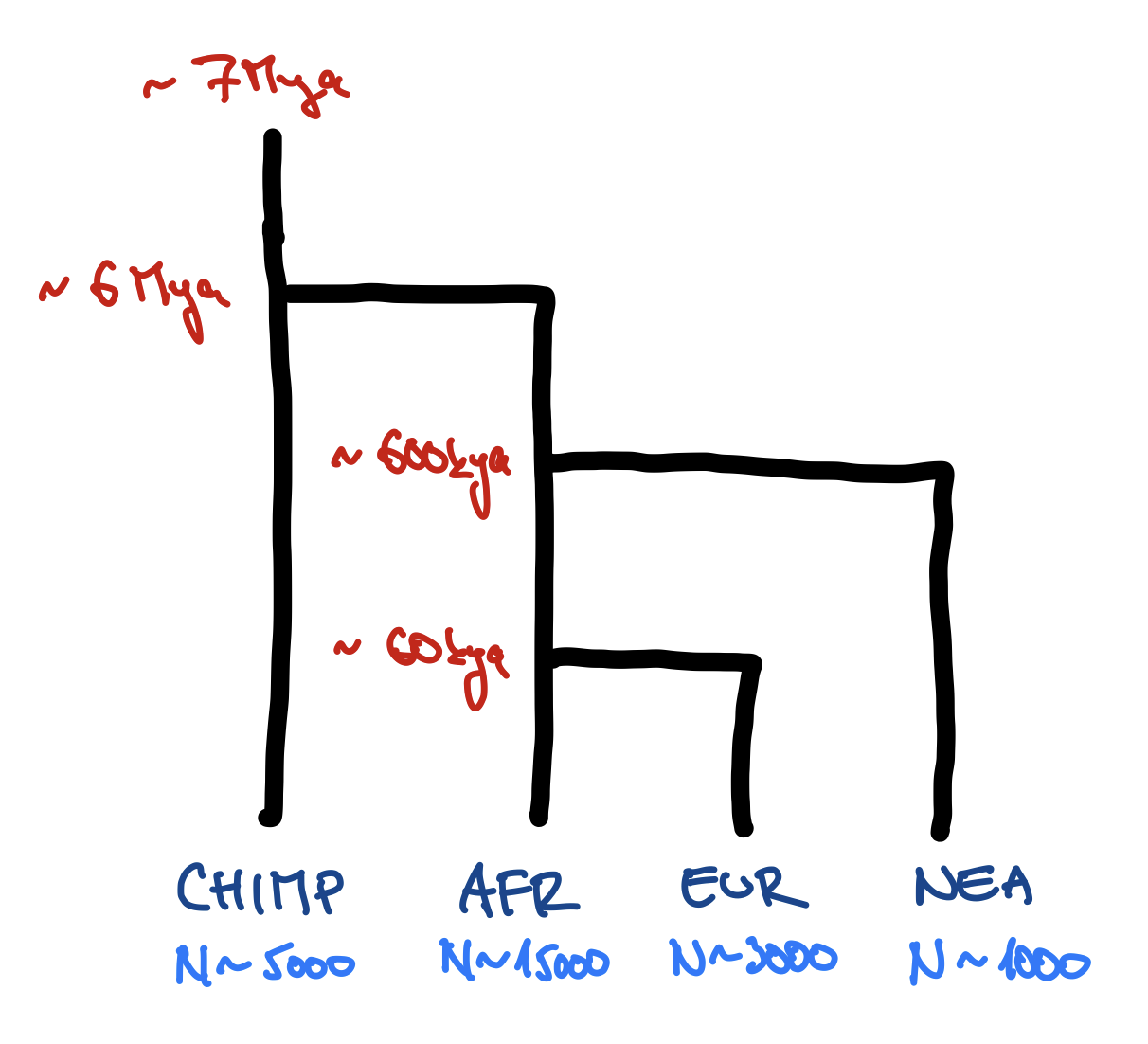

Don’t worry about gene flow just yet. We will add that at a later stage.

Feel free to include expansions and contractions (maybe in EUR at some point?).

Exercise #1 — solution

Simulating data (finally…)

We have a compiled model, how do we simulate data?

slendr has two built-in simulation engines:

SLiM engine
msprime engine

**You don’t have to write any msprime or SLiM code!**

This is all that’s needed:

ts <- msprime(model, sequence_length = 100e6, recombination_rate = 1e-8)

(ts is a so-called tree sequence)

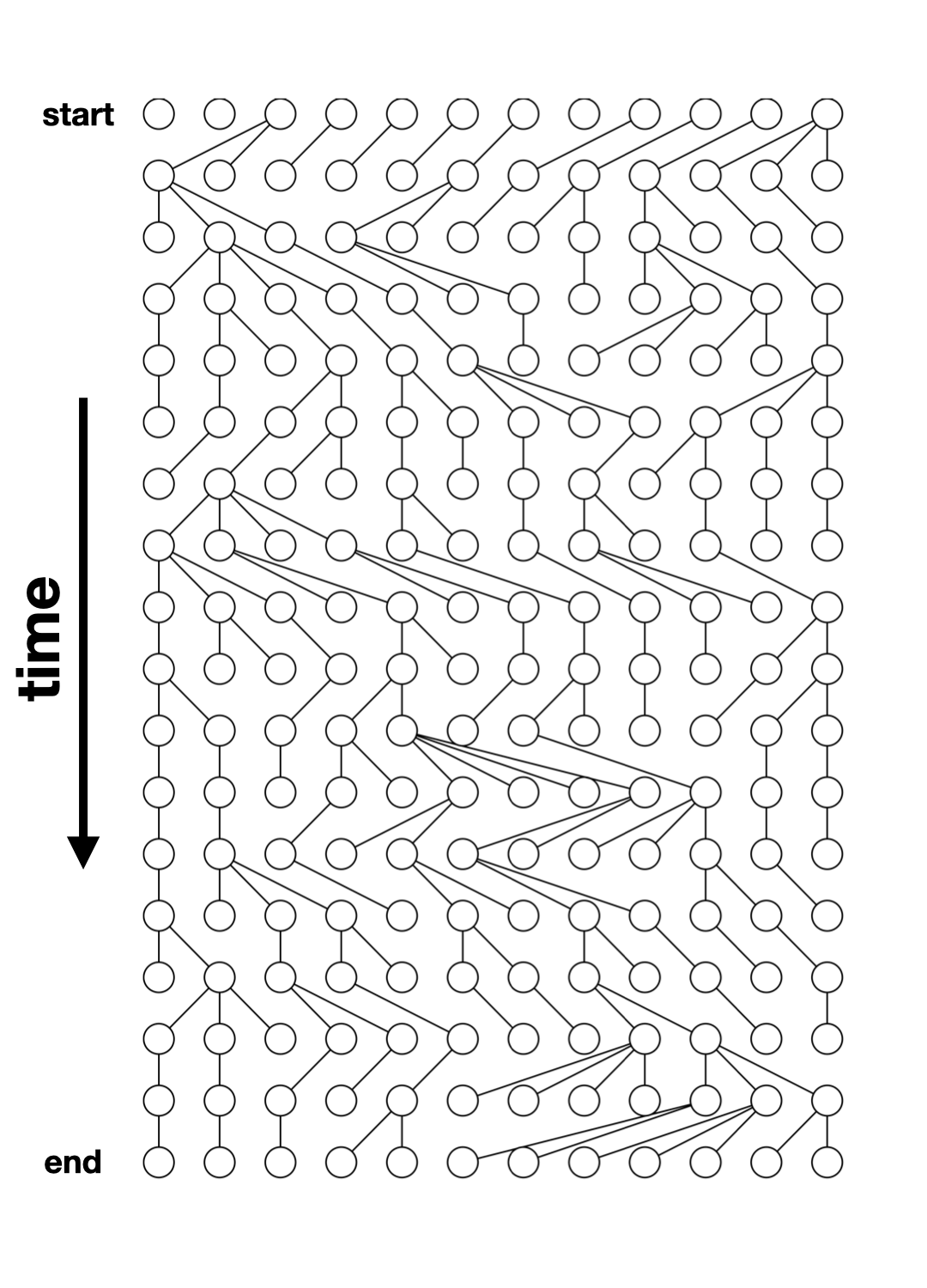
The output of a slendr simulation is a tree sequence

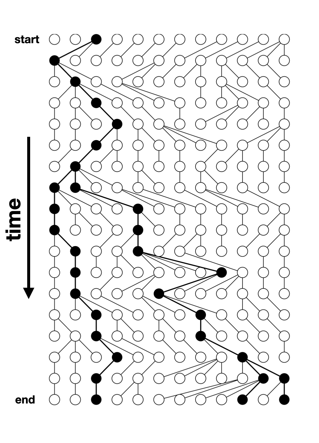
What is tree sequence?

a record of full genetic ancestry of a set of samples
an encoding of DNA sequence carried by those samples
an efficient analysis framework

Why tree sequence?

Why not VCF, EIGENSTRAT, or a genotype table?

What we usually have

What we usually want

(As full as possible) a representation of our samples’ history:

This is exactly what a tree sequence is.

Here is the magic

Tree sequences make it possible to directly compute many quantities of interest without going via conversion to a genotype table/VCF!

Ralph et al. (2020)

How can we compute statistics without mutations?

There is a duality between mutations and branch lengths in trees (more here).

But what if we want mutations?

Coalescent and mutation processes can be decoupled

This means we can add mutations
after the simulation.

This allows efficient, massive simulations

If we have a simulated ts object, we can do:

ts_mutated <- ts_mutate(ts, mutation_rate = 1e-8)

Or, with a shortcut:

ts <-
  msprime(model, sequence_length = 100e6, recombination_rate = 1e-8) %>%
  ts_mutate(mutation_rate = 1e-8 )

We will be using ts_mutate() throughout.

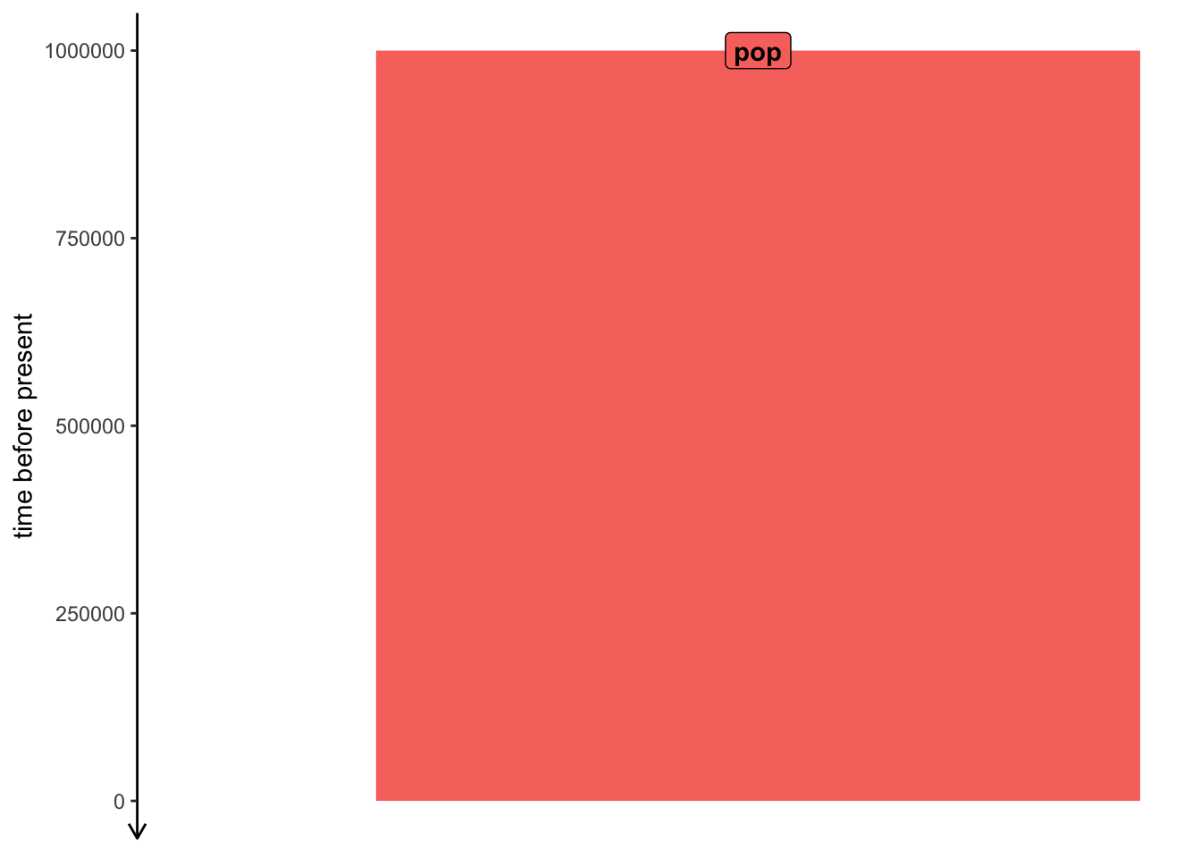
Tree sequences are also very efficient

Let’s take this minimalistic model:

pop <- population("pop", time = 1e6, N = 10000)
model <- compile_model(pop, generation_time = 30, direction = "backward")
ts <- msprime(model, sequence_length = 1e6, recombination_rate = 1e-8)

(simulates 2 \(\times\) 10000 chromosomes of 100 Mb)

Runs in less than 30 seconds on my laptop!

Taking about 66 Mb of memory!

How does this work?!

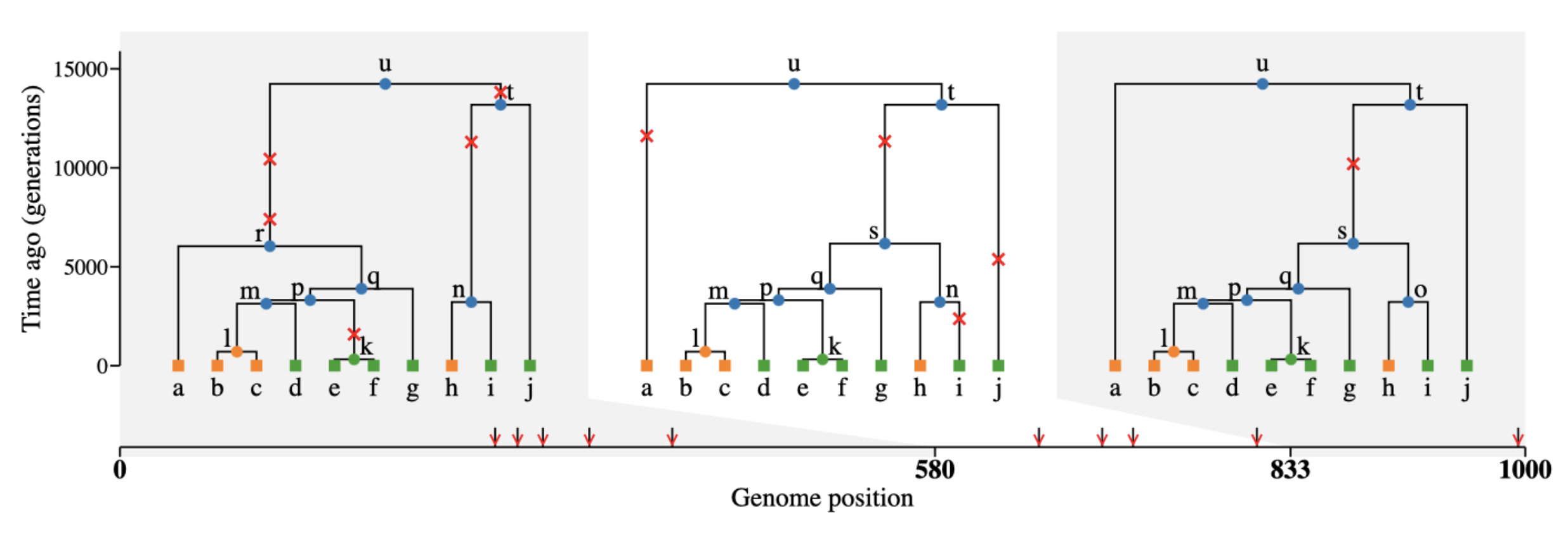
Tree-sequence tables (tskit docs)

A tree (sequence) can be represented by

a table of nodes,
a table of edges between nodes,
a table of mutations on edges

A set of such tables is a tree sequence.

Tree-sequence tables in practice

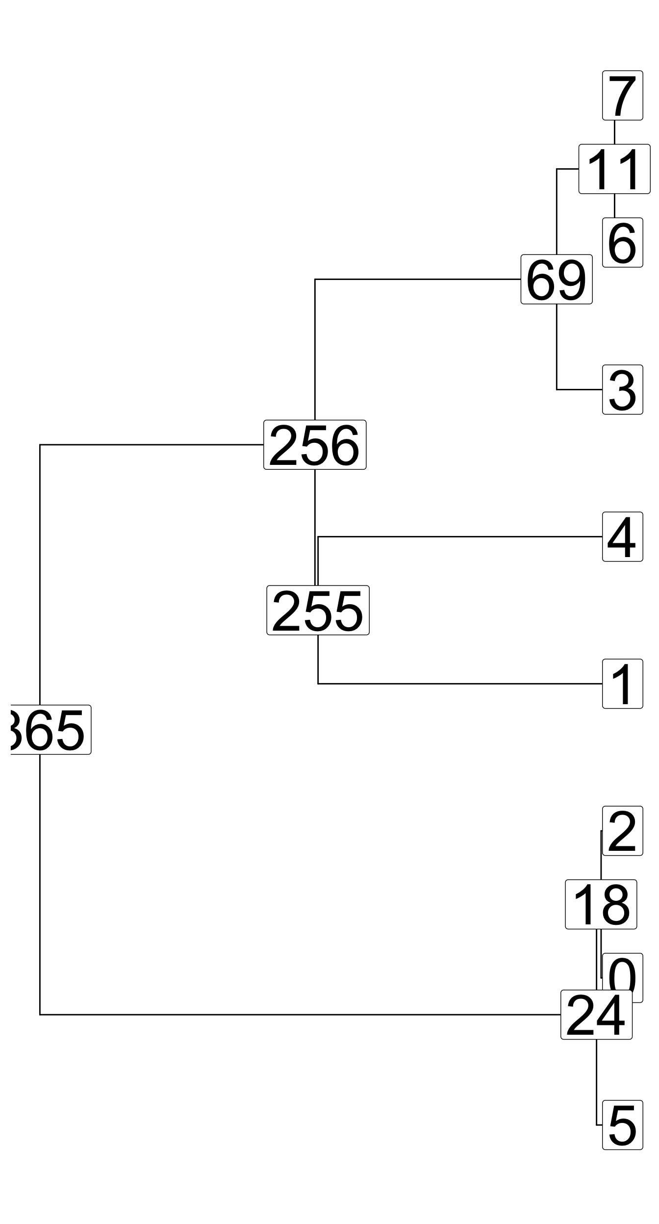
nodes:

  node_id pop_id     time
1     365      0 901433.1
2     256      0 475982.3
3     255      0 471179.5

edges:

  child_node_id parent_node_id
1           256            365
2           255            256
3            69            256

mutations:

[1] id   site node time
<0 rows> (or 0-length row.names)

Let’s take the `model` we defined earlier…

… and simulate tree sequence from it

ts <- msprime(model, sequence_length = 1e6, recombination_rate = 1e-8)

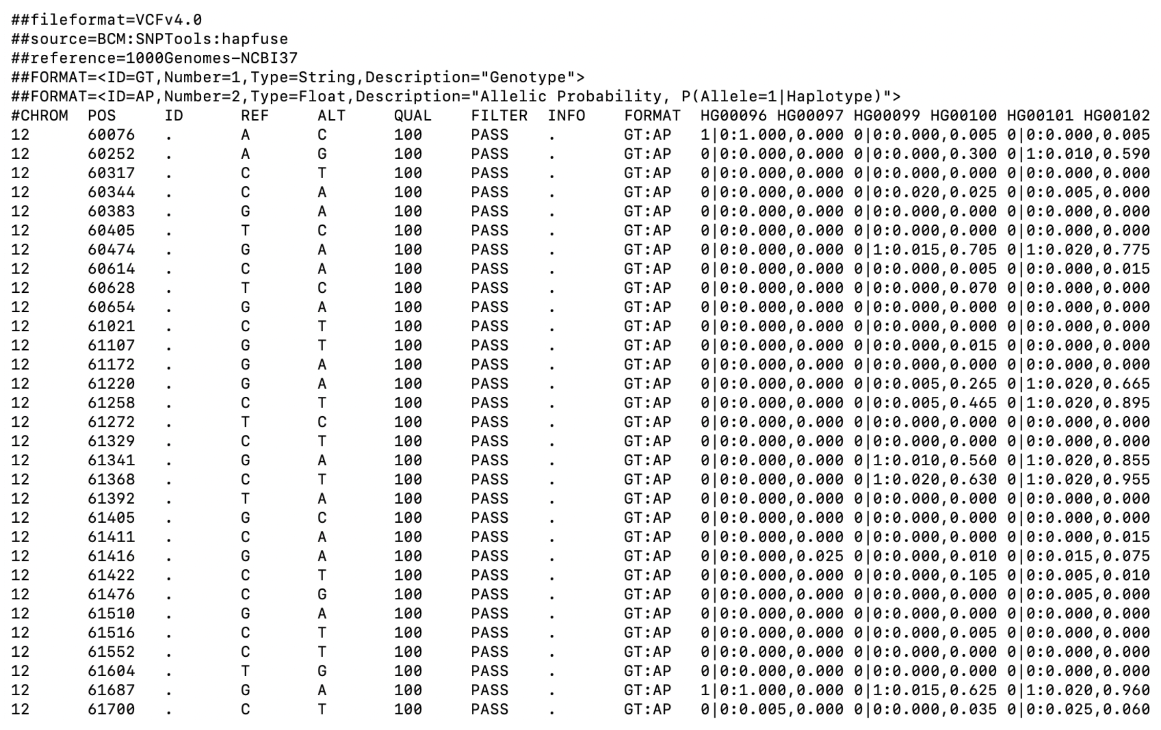
(A tree sequence can be saved to disk with ts_save().)

Conversion to other genotype formats

If you have a tree-sequence object ts, you can do…

ts_vcf(ts, path = "path/to/a/file.vcf.gz")

ts_eigenstrat(ts, prefix = "path/to/eigenstrat/prefix")

ts_genotypes(ts)

# A tibble: 935 × 7
     pos pop_1_chr1 pop_1_chr2 pop_2_chr1 pop_2_chr2 pop_3_chr1 pop_3_chr2
   <int>      <int>      <int>      <int>      <int>      <int>      <int>
 1   670          0          0          0          0          0          1
 2   790          0          0          0          1          0          0
 3  3525          1          0          1          0          0          0
 4  4224          0          1          0          0          1          0
 5  7036          1          0          1          0          0          0
 6  8019          1          0          1          0          0          0
 7  9063          0          1          0          1          1          1
 8  9961          1          1          1          0          1          0
 9 10623          0          0          0          1          0          1
10 12526          1          1          1          0          1          0
# … with 925 more rows

What can we do with it?

slendr’s R interface to tskit

This R interface links to Python methods implemented in tskit.

Extracting sample information

Each “sampled” individual in slendr has a symbolic name, a sampling time, and a population assignment.

Extracting sample information

If we have a tree sequence ts, we can get samples with ts_samples():

ts_samples(ts)

# A tibble: 3 × 3
  name   time pop  
  <chr> <dbl> <chr>
1 pop_1     0 pop  
2 pop_2     0 pop  
3 pop_3     0 pop

ts_samples(ts) %>% count(pop)

# A tibble: 1 × 2
  pop       n
  <chr> <int>
1 pop       3

Analyzing tree sequences with slendr

Let’s say we have the following model and we simulate a tree sequence from it.

pop <- population("pop", N = 10000, time = 1)

model <- compile_model(pop, generation_time = 1, simulation_length = 10000)

ts <-
  msprime(model, sequence_length = 100e6, recombination_rate = 1e-8) %>%
  ts_mutate(mutation_rate = 1e-8)

Imagine we want to get the allele-frequency spectrum.

Example: allele frequency spectrum

# sample 5 individuals
samples <-
  ts_samples(ts) %>%
  sample_n(5) %>%
  pull(name)

samples

[1] "pop_2369" "pop_5273" "pop_9290" "pop_1252" "pop_8826"

# compute the AFS
afs <- ts_afs(
  ts, list(samples),
  polarised = TRUE
)

afs

 [1] 39887 19809 13465 10387  8024  6634  5543  5134  4567  3888

plot(afs, type = "b",
     xlab = "allele count bin",
     ylab = "frequency")

Exercise #2

Exercise #2 — estimating \(N_e\) from AFS

You sequenced 10 individuals from one population and computed this AFS (counts of singletons, doubletons, …):

afs_observed <- c(2520, 1449, 855, 622, 530, 446, 365, 334, 349, 244,
                  264, 218,  133, 173, 159, 142, 167, 129, 125, 143)

You know from fossil evidence that the population had constant \(N_e\) for the past 100,000 generations, and that the \(N_e\) was somewhere between 1000 and 30000.

Use slendr to guess the true value of \(N_e\) given the observed AFS by running single-population simulations of different \(N_e\) and comparing ts_afs() results to afs_observed.

Exercise #2 – hints

Write an R function (in a new script) that gets \(N_e\) as input, creates a slendr population, compiles a model, simulates a tree sequence, runs ts_afs() on it, and returns the AFS.
Find the \(N_e\) value that will give the closest AFS to the observed one. For instance, you could:
- a ) Plot simulated AFS for different \(N_e\) with the AFS and just eyeball \(N_e\) value that looks correct from a graph.
- b ) Simulate AFS automatically in steps of possible \(N_e\) values and find the closest matching one.

Exercise #2 solution (a) – eye-balling

Exercise #2 solution (b) – grid

Gene flow / admixture

`gene_flow()` events

Gene flow is programmed the gene_flow() function.

If we have populations p1 and p2, we schedule gene flow with:

gf <- gene_flow(from = p1, to = p2, start = 500, end = 600, rate = 0.13)

Multiple gene-flow events can be gathered in a list:

gf <- list(
  gene_flow(from = p1, to = p2, start = 500, end = 600, rate = 0.13),
  gene_flow(from = <..>, to = <..>, start = <...>, end = <...>, rate = <...>),
  < potentially many more ... >
)

gene_flow() checks for consistency!

Plugging gene flow(s) into the model

gf <- gene_flow(from = ..., to = ..., <start, end, rate>)

model <- compile_model(
  populations = list(...),
  gene_flow = gf,           # <--- gene flow(s) specified
  generation_time = 30
)

Exercise #3

Exercise #3 — adding `gene_flow()`

Add Neanderthal introgression into your model from Exercise #1 (let’s say 3% pulse NEA -> EUR at 55 kya).

Exercise #3 — adding `gene_flow()`

Add Neanderthal introgression into your model from Exercise #1 (let’s say 3% pulse NEA -> EUR at 55 kya).

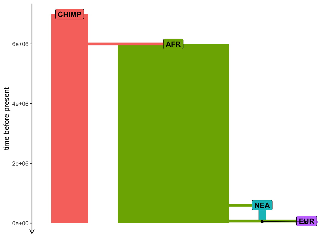
Exercise #3 — solution

Exercise #4

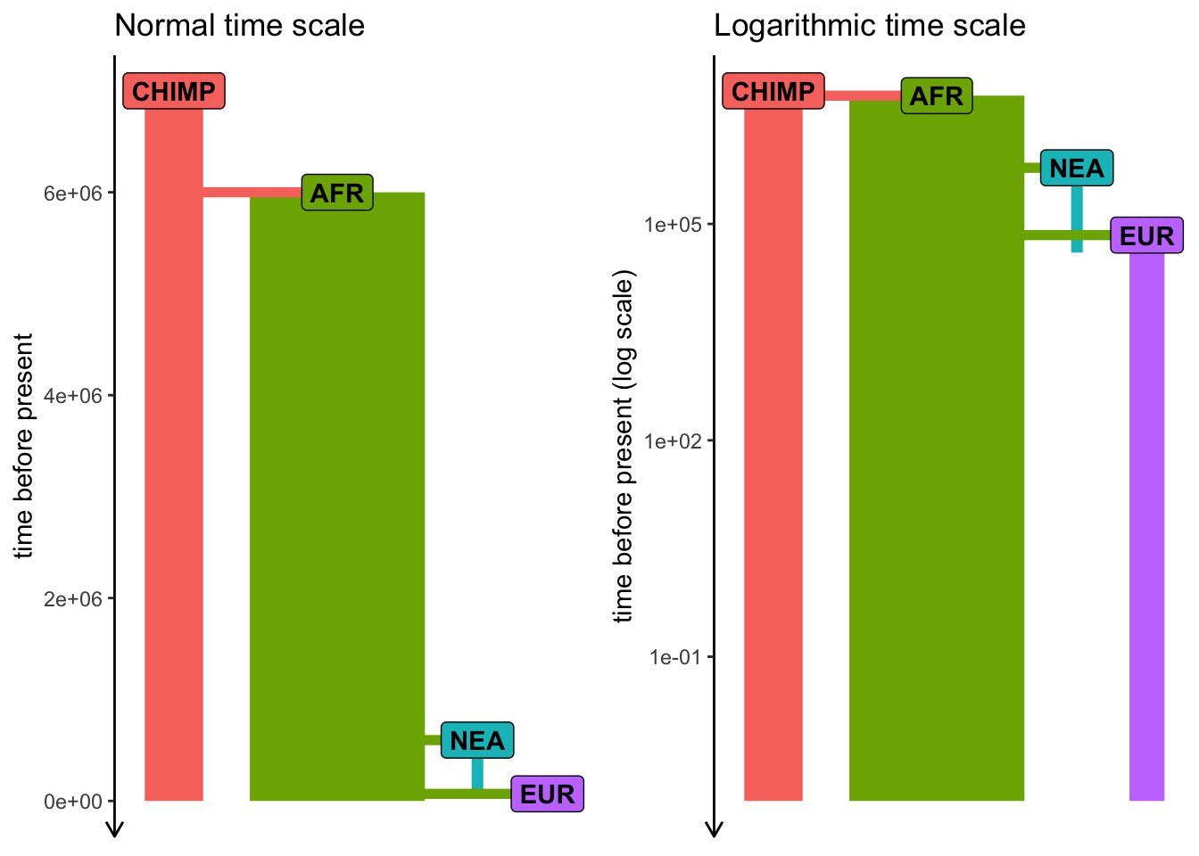
Exercise #4 — popgen statistics

plot_model(model)

Exercise #4 — popgen statistics

Compute nucleotide diversity (\(\pi\)) in each population (ts_diversity()). Do your results with known \(N_e\) values?

Compute ts_divergence() (genetic divergence) or ts_fst() (\(F_{ST}\)) between populations. Do the results match the model?

Compute the “outgroup \(f_3\)” using CHIMP as the outgroup (ts_f3()) for different pairs of “A” and “B” populations.

Test Neanderthal introgression in EUR using the \(f_4\) statistic (ts_f4()). [hint: \(f_4\)(AFR, EUR; NEAND, CHIMP)]

Exercise #4 — popgen statistics

A useful R trick for handling recorded samples:

ts_samples(ts)

# A tibble: 24,000 × 3
   name    time pop  
   <chr>  <dbl> <chr>
 1 AFR_1      0 AFR  
 2 AFR_2      0 AFR  
 3 AFR_3      0 AFR  
 4 AFR_4      0 AFR  
 5 AFR_5      0 AFR  
 6 AFR_6      0 AFR  
 7 AFR_7      0 AFR  
 8 AFR_8      0 AFR  
 9 AFR_9      0 AFR  
10 AFR_10     0 AFR  
# … with 23,990 more rows

samples <- ts_samples(ts) %>%
  split(., .$pop) %>%
  lapply(pull, "name")

str(samples)

List of 4
 $ AFR  : chr [1:15000] "AFR_1" "AFR_2" "AFR_3" "AFR_4" ...
 $ CHIMP: chr [1:5000] "CHIMP_1" "CHIMP_2" "CHIMP_3" "CHIMP_4" ...
 $ EUR  : chr [1:3000] "EUR_1" "EUR_2" "EUR_3" "EUR_4" ...
 $ NEA  : chr [1:1000] "NEA_1" "NEA_2" "NEA_3" "NEA_4" ...

Exercise #4 — solution

Time-series data

Sampling aDNA samples through time

Imagine we have pop1, pop2, … compiled in a model.

To record ancient individuals in the tree sequence, we can use schedule_sampling() like this:

schedule_sampling(
  model,                # compiled slendr model object
  times = c(100, 500),  # at these times (can be also a single number) ...
  list(pop1, 42),       # ... sample 42 individuals from pop1
  list(pop2, 10),       # ... sample 10 individuals from pop2
  list(pop3, 1)         # ... sample 1 individual from pop 3
)

Sampling schedule format

The output of schedule_sampling() is a plain data frame:

schedule_sampling(model, times = c(40000, 30000, 20000, 10000), list(eur, 1))

# A tibble: 4 × 7
   time pop       n y_orig x_orig y     x    
  <int> <chr> <int> <lgl>  <lgl>  <lgl> <lgl>
1 10000 EUR       1 NA     NA     NA    NA   
2 20000 EUR       1 NA     NA     NA    NA   
3 30000 EUR       1 NA     NA     NA    NA   
4 40000 EUR       1 NA     NA     NA    NA

We can bind multiple sampling schedules together, giving us finer control about sampling:

eur_samples <- schedule_sampling(model, times = c(40000, 30000, 20000, 10000, 0), list(eur, 1))
afr_samples <- schedule_sampling(model, times = 0, list(afr, 1))

samples <- bind_rows(eur_samples, afr_samples)

How to use a sampling schedule?

To sample individuals based on a given schedule, we use the samples = argument of the msprime() functions:

ts <- msprime(model, samples = samples, sequence_length = 1e6, recombination_rate = 1e-8) %>% 
  ts_mutate(mutation_rate = 1e-8)

We can verify that only specific individuals are recorded:

ts_samples(ts)

# A tibble: 6 × 3
  name   time pop  
  <chr> <dbl> <chr>
1 EUR_1 40000 EUR  
2 EUR_2 30000 EUR  
3 EUR_3 20000 EUR  
4 EUR_4 10000 EUR  
5 AFR_1     0 AFR  
6 EUR_5     0 EUR

ts

╔═══════════════════════════╗
║TreeSequence               ║
╠═══════════════╤═══════════╣
║Trees          │       1189║
╟───────────────┼───────────╢
║Sequence Length│    1000000║
╟───────────────┼───────────╢
║Time Units     │generations║
╟───────────────┼───────────╢
║Sample Nodes   │         12║
╟───────────────┼───────────╢
║Total Size     │  264.9 KiB║
╚═══════════════╧═══════════╝
╔═══════════╤════╤═════════╤════════════╗
║Table      │Rows│Size     │Has Metadata║
╠═══════════╪════╪═════════╪════════════╣
║Edges      │3616│113.0 KiB│          No║
╟───────────┼────┼─────────┼────────────╢
║Individuals│   6│192 Bytes│          No║
╟───────────┼────┼─────────┼────────────╢
║Migrations │   0│  8 Bytes│          No║
╟───────────┼────┼─────────┼────────────╢
║Mutations  │1580│ 57.1 KiB│          No║
╟───────────┼────┼─────────┼────────────╢
║Nodes      │ 858│ 23.5 KiB│          No║
╟───────────┼────┼─────────┼────────────╢
║Populations│   4│341 Bytes│         Yes║
╟───────────┼────┼─────────┼────────────╢
║Provenances│   2│  3.5 KiB│          No║
╟───────────┼────┼─────────┼────────────╢
║Sites      │1579│ 38.6 KiB│          No║
╚═══════════╧════╧═════════╧════════════╝

Exercise #5

Exercise #5a — ancient samples

Simulate data from your model using this sampling:

one present-day CHIMP and AFR individual
20 present-day EUR individuals
1 NEA at 70 ky, 1 NEA at 40 ky
1 EUR every 1000 years between 50-5 kya

Reminder: you can do this by:

samples <- # rbind(...) together individual schedule_sampling() data frames

ts <-
  msprime(model, samples = samples, sequence_length = 100e6, recombination_rate = 1e-8) %>%
  ts_mutate(mutation_rate = 1e-8)

Exercise #5b — \(f_4\)-ratio statistic

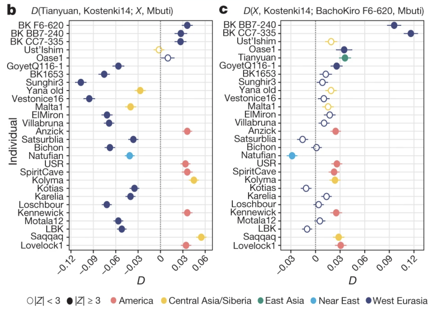
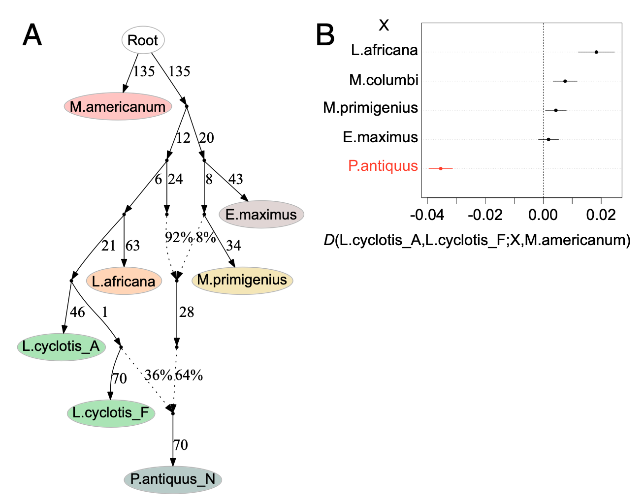
Use \(f_4\)-ratio statistic to replicate the following figure:

Hint: You can compute Neanderthal ancestry for a vector of individuals X as ts_f4ratio(ts, X = X, "NEA_1", "NEA_2", "AFR_1", "CHIMP_1").

Exercise #5 — solution

More information

slendr paper on bioRxiv
Documentation, tutorials can be found here
GitHub repo (bug reports!) is here

new R package for ABC modeling demografr

Why use simulations?

Making sense of estimated statistics

Making sense of estimated statistics

Making sense of estimated statistics

Fitting model parameters (i.e. ABC)

Ground truth for methods work

There are many simulation tools

SLiM

What is SLiM?

SLiMgui – IDE for SLiM

Simple neutral simulation in SLiM

msprime

What is msprime?

What is msprime?

Simple simulation using msprime

www.slendr.net

Why a new package? – spatial simulations!

Why a new package?

Let’s get started

We will need slendr & tidyverse

slendr haiku

Typical steps (outline of this tutorial)

Creating a population()

Programming population splits

Scheduling resize events – resize()

Tidyverse-style pipe %>% interface

A more complex model

Remember that slendr objects internally carry their whole history!

Last step before simulation: compile_model()

Model summary

Model visualization

Exercise #1

Exercise #1 — write your own model!

Exercise #1 — solution

Simulating data (finally…)

You don’t have to write any msprime or SLiM code!

The output of a slendr simulation is a tree sequence

What is tree sequence?

Why tree sequence?

Why not VCF, EIGENSTRAT, or a genotype table?

What we usually have

What we usually want

Here is the magic

How can we compute statistics without mutations?

But what if we want mutations?

Coalescent and mutation processes can be decoupled

This means we can add mutationsafter the simulation.

This allows efficient, massive simulations

Tree sequences are also very efficient

How does this work?!

Tree-sequence tables (tskit docs)

A set of such tables is a tree sequence.

Tree-sequence tables in practice

Let’s take the model we defined earlier…

… and simulate tree sequence from it

Conversion to other genotype formats

What can we do with it?

slendr’s R interface to tskit

Extracting sample information

Extracting sample information

Analyzing tree sequences with slendr

Example: allele frequency spectrum

Exercise #2

Exercise #2 — estimating \(N_e\) from AFS

Exercise #2 – hints

Exercise #2 solution (a) – eye-balling

Exercise #2 solution (b) – grid

Gene flow / admixture

gene_flow() events

Plugging gene flow(s) into the model

Exercise #3

Exercise #3 — adding gene_flow()

Exercise #3 — adding gene_flow()

Exercise #3 — solution

Exercise #4

Exercise #4 — popgen statistics

Exercise #4 — popgen statistics

Exercise #4 — popgen statistics

Exercise #4 — solution

Time-series data

Creating a `population()`

Scheduling resize events – `resize()`

Tidyverse-style pipe `%>%` interface

Last step before simulation: `compile_model()`

**You don’t have to write any msprime or SLiM code!**

This means we can add mutations
after the simulation.

Let’s take the `model` we defined earlier…

`gene_flow()` events

Exercise #3 — adding `gene_flow()`

Exercise #3 — adding `gene_flow()`