Simulations in population genetics

PopGen summer course 2023

Martin Petr

August 2023

First things first

These slides and other resources are (and always will be) at:

github.com/bodkan/ku-popgen2023


Open this link now so you have everything at hand later.

Many problems in population genetics cannot be solved by a mathematician, no matter how gifted. [It] is already clear that computer methods are very powerful. This is good. It […] permits people with limited mathematical knowledge to work on important problems […].

Why use simulations?

  1. Making sense of inferred statistics
  2. Fitting model parameters (i.e. ABC)
  3. Ground truth for method development

Making sense of inferred statistics

Making sense of inferred statistics

Fitting model parameters (i.e. ABC)

Ground truth for method development

What does it mean to simulate a genome?


How would you design an algorithm for a popgen simulation?


What minimum components are needed?

If we want to simulate population genetics


We need populations.

We need genetics.

The ‘genetics’ part…


…a linear sequence of nucleotides (a chromosome)

  • a list of characters (A/G/C/T nucleotides)
  • a list of 0 or 1 values (ancestral/derived allele),

which (maybe) mutates at a given mutation rate,

and (maybe) recombines at a certain recombination rate.

The ‘population’ part…


… a collection of individuals at a given point in time,

each carrying chromosomes inherited from its parents.

Single-locus
Wright-Fisher
simulation in R


“What is the expected trajectory of a neutral allele under the influence of genetic drift?”

From Fernando’s lecture on Monday…


A complete Wright-Fisher simulation

p_0 <- 0.5  # initial allele frequency ("50% marbles" from lecture #1)
N   <- 500  # number of chromosomes in a population
T   <- 2000 # number of generations to simulate

# a vector for storing frequencies over time
p_trajectory <- p_0 

# in each generation:
for (gen_i in 2:T) {
  # get frequency in the previous generation
  p_prev <- p_trajectory[gen_i - 1] 

  # calculate new frequency ("sampling marbles from a jar")
  p_trajectory[gen_i] <- rbinom(1, N, p_prev) / N 
}

plot(p_trajectory)

\(N\) = 500, \(p_0 = 0.5\)

Code
plot(p_trajectory, type = "l", ylim = c(0, 1),
     xlab = "generations", ylab = "allele frequency")
abline(h = p_0, lty = 2, col = "red")

Let’s make it a function

Input: \(p_0\), \(N\), and the number of generations

Output: allele frequency trajectory vector

simulate <- function(p_0, N, T) {
  p_trajectory <- p_0

  for (gen_i in 2:T) {
    p_prev <- p_trajectory[gen_i - 1]
    p <- rbinom(1, N, p_prev) / N
    p_trajectory[gen_i] <- p
  }

  return(p_trajectory)
}

And then:

simulate(p_0 = 0.5, N = 1000, T = 10)
 [1] 0.500 0.476 0.464 0.458 0.435 0.449 0.464 0.465 0.466 0.462

\(N\) = 500, \(p_0 = 0.5\) (20 replicates)

Code
reps <- replicate(20, simulate(N = 500, p_0 = 0.5, T = 2000))

matplot(reps, ylim = c(0, 1), xlab = "generations", ylab = "allele frequency", type = "l", lty = 1)

\(N\) = 1000, \(p_0 = 0.5\) (20 replicates)

Code
reps <- replicate(20, simulate(N = 1000, p_0 = 0.5, T = 2000))

matplot(reps, ylim = c(0, 1), xlab = "generations", ylab = "allele frequency", type = "l", lty = 1)

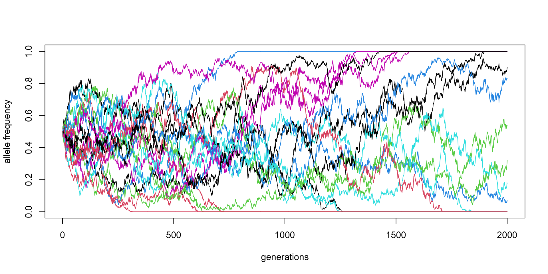
\(N\) = 5000, \(p_0 = 0.5\) (20 replicates)

Code
reps <- replicate(20, simulate(N = 5000, p_0 = 0.5, T = 2000))

matplot(reps, ylim = c(0, 1), xlab = "generations", ylab = "allele frequency", type = "l", lty = 1)

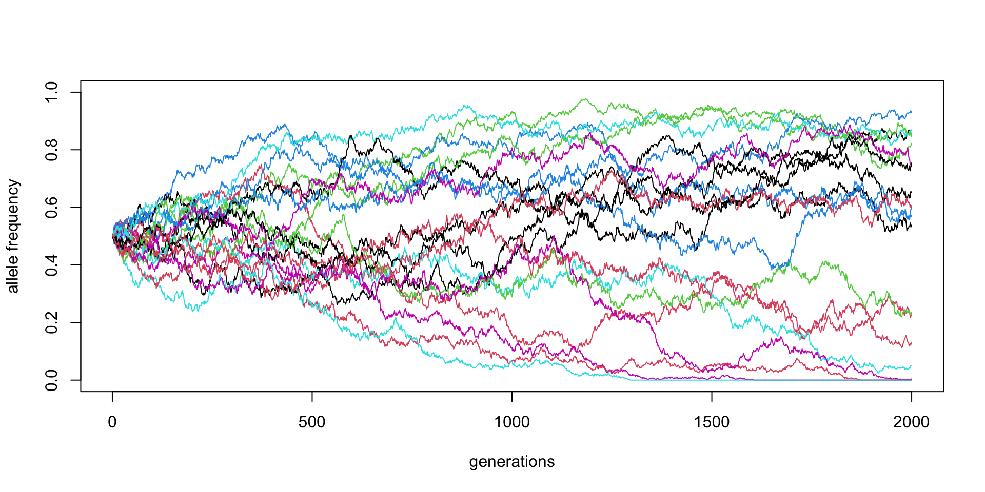
\(N\) = 10000, \(p_0 = 0.5\) (20 replicates)

Code
reps <- replicate(20, simulate(N = 10000, p_0 = 0.5, T = 2000))

matplot(reps, ylim = c(0, 1), xlab = "generations", ylab = "allele frequency", type = "l", lty = 1)

\(N\) = 10000, \(p_0 = 0.5\) (100 replicates)

Code
reps <- replicate(100, simulate(N = 10000, p_0 = 0.5, T = 30000))

matplot(reps, ylim = c(0, 1), xlab = "generations", ylab = "allele frequency", type = "l", lty = 1)

\(N\) = 10000, \(p_0 = 0.5\) (100 replicates)

Code
factors <- MASS::fractions(c(3, 2, 1, 1/2, 1/5, 1/10))
matplot(reps, ylim = c(0, 1), xlab = "generations", ylab = "allele frequency", type = "l", lty = 1)
abline(v = 10000 * factors, lwd = 5)

Expected allele frequency distribution

Code
library(ggplot2)
library(dplyr)
library(parallel)

if (!file.exists("diffusion.rds")) {
p_0 <- 0.5
N <- 10000
factors <- MASS::fractions(c(3, 2, 1, 1/2, 1/5, 1/10))

final_frequencies <- parallel::mclapply(
  seq_along(factors), function(i) {
    f <- factors[i]
    t <- as.integer(N * f)
    # get complete trajectories as a matrix (each column a single trajectory)
    reps <- replicate(10000, simulate(N = N, p_0 = p_0, T = t))
    # only keep the last slice of the matrix with the final frequencies
    data.frame(
      t = sprintf("t = %s * N", f),
      freq = reps[t, ]
    )
  },
  mc.cores = parallel::detectCores()
) %>% do.call(rbind, .)
final_frequencies$t <- forcats::fct_rev(forcats::fct_relevel(final_frequencies$t, sprintf("t = %s * N", factors)))
saveRDS(final_frequencies, "diffusion.rds")
} else {
  final_frequencies <- readRDS("diffusion.rds")
}

final_frequencies %>% .[.$freq > 0 & .$freq < 1, ] %>%
ggplot() +
  geom_histogram(aes(freq, y = after_stat(density), fill = t), position = "identity", bins = 100, alpha = 0.75) +
  labs(x = "allele frequency") +
  coord_cartesian(ylim = c(0, 3)) +
  facet_grid(t ~ .) +
  guides(fill = guide_legend(sprintf("time since\nthe start\n[assuming\nN = %s]", N))) +
  theme_minimal() +
  theme(strip.text.y = element_blank(),
        axis.title.x = element_text(size = 15),
        axis.title.y = element_text(size = 15),
        axis.text.x = element_text(size = 15),
        axis.text.y = element_text(size = 15),
        legend.title = element_text(size = 15),
        legend.text = element_text(size = 15))

“Diffusion Models in Population Genetics”, Kimura (1964)


  But now for something
  completely different.


  Let’s talk about
  real simulations.

There are many simulation tools

The most famous and widely used are SLiM and msprime.

They are very powerful but both require:

  • quite a bit of programming knowledge,
  • a lot of code for non-trivial simulations (🐛🪲🐜).


The exercises will focus on the slendr
popgen simulation toolkit for R.


But let’s look at SLiM and msprime at least a little bit.

What is SLiM?

  • A forward-time simulator
  • It’s fully programmable!
  • Massive library of functions for:
    • demographic events
    • various mating systems
    • selection, quantitative traits, …

Modified from Alexei Drummond

Simple neutral simulation in SLiM

initialize() {
    // create a neutral mutation type
    initializeMutationType("m1", 0.5, "f", 0.0);
    // initialize 1Mb segment
    initializeGenomicElementType("g1", m1, 1.0);
    initializeGenomicElement(g1, 0, 999999);
    // set mutation rate and recombination rate of the segment
    initializeMutationRate(1e-8);
    initializeRecombinationRate(1e-8);
}

// create an ancestral population p1 of 10000 diploid individuals
1 early() { sim.addSubpop("p1", 10000); }

// in generation 1000, create two daughter populations p2 and p3
1000 early() {
    sim.addSubpopSplit("p2", 5000, p1);
    sim.addSubpopSplit("p3", 1000, p1);
}

// in generation 10000, stop the simulation and save 100 individuals
// from p2 and p3 to a VCF file
10000 late() {
    p2_subset = sample(p2.individuals, 100);
    p3_subset = sample(p3.individuals, 100);
    c(p2_subset, p3_subset).genomes.outputVCF("/tmp/slim_output.vcf.gz");
    sim.simulationFinished();
    catn("DONE!");
}

What is msprime?

  • A Python module for writing coalescent simulations
  • Extremely fast (genome-scale, population-scale data)
  • You must know Python fairly well to build complex models

Modified from Alexei Drummond

Simple simulation using msprime

import msprime

demography = msprime.Demography()
demography.add_population(name="A", initial_size=10_000)
demography.add_population(name="B", initial_size=5_000)
demography.add_population(name="C", initial_size=1_000)
demography.add_population_split(time=1000, derived=["A", "B"], ancestral="C")

ts = msprime.sim_ancestry(
  sequence_length=10e6,
  recombination_rate=1e-8,
  samples={"A": 100, "B": 100},
  demography=demography
)

www.slendr.net

Why a new package?

Spatial simulations!

Why a new package?

  • Most researchers are not expert programmers

  • All but the most trivial simulations require lots of code

  • 90% [citation needed] of simulations are basically the same!

    • create populations (splits and \(N_e\) changes)

    • specify if/how they should mix (rates and times)

  • Lot of code duplication across projects
slendr makes “standard” demographic simulations trivial
and unlocks new kinds of spatial simulations

Let’s get started

Everything we do will be in R


Always start your R scripts with this (*):

library(slendr)
init_env()


My solutions will also use these two packages:

library(ggplot2)
library(dplyr)

Typical steps of a slendr R workflow


  1. creating populations
  2. scheduling population splits
  3. programming \(N_e\) size changes
  4. encoding gene-flow events
  5. simulation sequence of a given size
  6. computing statistics from simulated outputs

Creating a population()

Each needs a name, size and time of appearance:

pop1 <- population("pop1", N = 1000, time = 1)


This creates a normal R object. Typing it out gives a summary:

pop1
slendr 'population' object 
-------------------------- 
name: pop1 
non-spatial population
stays until the end of the simulation

population history overview:
  - time 1: created as an ancestral population (N = 1000)

Programming population splits

Splits are indicated by the parent = <pop> argument:

pop2 <- population("pop2", N = 100, time = 50, parent = pop1)


The split is reported in the “historical summary”:

pop2
slendr 'population' object 
-------------------------- 
name: pop2 
non-spatial population
stays until the end of the simulation

population history overview:
  - time 50: split from pop1 (N = 100)

Scheduling resize events – resize()

Step size decrease:

pop1 <- population("pop1", N = 1000, time = 1)
pop1_step <- resize(pop1, N = 100, time = 500, how = "step")


Exponential increase:

pop2 <- population("pop2", N = 100, time = 50, parent = pop1)
pop2_exp <- resize(pop2, N = 10000, time = 500, end = 2000, how = "exponential")

Tidyverse-style pipe %>% interface

A more concise way to express the same thing as before.


Step size decrease:

pop1 <-
  population("pop1", N = 1000, time = 1) %>%
  resize(N = 100, time = 500, how = "step")


Exponential increase:

pop2 <-
  population("pop2", N = 1000, time = 1) %>%
  resize(N = 10000, time = 500, end = 2000, how = "exponential")

A more complex model

pop1 <- population("pop1", N = 1000, time = 1)

pop2 <-
  population("pop2", N = 1000, time = 300, parent = pop1) %>%
  resize(N = 100, how = "step", time = 1000)

pop3 <-
  population("pop3", N = 1000, time = 400, parent = pop2) %>%
  resize(N = 2500, how = "step", time = 800)

pop4 <-
  population("pop4", N = 1500, time = 500, parent = pop3) %>%
  resize(N = 700, how = "exponential", time = 1200, end = 2000)

pop5 <-
  population("pop5", N = 100, time = 600, parent = pop4) %>%
  resize(N = 50, how = "step", time = 900) %>%
  resize(N = 1000, how = "exponential", time = 1600, end = 2200)

Each object carries its history!

pop5
slendr 'population' object 
-------------------------- 
name: pop5 
non-spatial population
stays until the end of the simulation

population history overview:
  - time 600: split from pop4 (N = 100)
  - time 900: resize from 100 to 50 individuals
  - time 1600-2200: exponential resize from 50 to 1000 individuals

Gene flow / admixture

We can schedule gene_flow() from pop1 into pop2 with:

gf <- gene_flow(from = pop1, to = pop2, start = 2000, end = 2200, rate = 0.13)

Here rate = 0.13 means 13% migrants over the given time window will come from “pop1” into “pop2”.


Multiple gene-flow events can be gathered in a list:

gf <- list(
  gene_flow(from = pop1, to = pop2, start = 500, end = 600, rate = 0.13),
  gene_flow(from = ..., to = ..., start = ..., end = ..., rate = ...),
  ...
)

Last step before simulation: compile_model()


model <- compile_model(
  list(pop1, pop2, pop3, pop4, pop5),
  generation_time = 1,
  simulation_length = 3000,
  direction = "forward"
)


Compilation takes a list of model components, performs internal consistency checks, returns a single model object.

Last step before simulation: compile_model()


model <- compile_model(
  list(pop1, pop2, pop3, pop4, pop5),
  gene_flow = gf,      # <----- in case our model includes gene flow
  generation_time = 1,
  simulation_length = 3000,
  direction = "forward"
)


Gene flow(s) that we programmed are included
via the gene_flow argument.

Model summary

Typing the compiled model into R prints a brief summary:

model
slendr 'model' object 
--------------------- 
populations: pop1, pop2, pop3, pop4, pop5 
geneflow events: 1 
generation time: 1 
time direction: forward 
total running length: 3000 model time units
model type: non-spatial

configuration files in: /private/var/folders/d_/hblb15pd3b94rg0v35920wd80000gn/T/RtmpyYatVY/fileaef453c85ae 

Model visualization

plot_model(model, proportions = TRUE)

Exercise #1

Go to the lecure & exercises page

Link: github.com/bodkan/ku-popgen2023

Open the relevant red-highlighted links:

Exercise #1: write this model in slendr

Start a model1.R script in RStudio with this “template”:

library(slendr); init_env()

<... population definitions ...>
<... gene flow definition ...>

model <- compile_model(
  populations = list(...),
  gene_flow = <...>,
  generation_time = 30
)

plot_model(model) # verify visually

Exercise #1 (bonus): your own model


Program a model for an organism that you study.


If applicable, include bottlenecks, expansions, etc. Don’t hesitate to make it as complex as you want.


Use plot_model() to check your model visually.


Save it in a different R script—you will use it in a later exercise.

Exercise #1: solution


So, now we can
write a model

How do we simulate from it?

slendr has two built-in simulation “engine scripts”:

They are designed to understand slendr models.


All you need to simulate data is this one line of code:

ts <- msprime(model, sequence_length = 100e6, recombination_rate = 1e-8)


You don’t have to write msprime or SLiM code!

The output of a slendr simulation is a tree sequence (ts)

What is tree sequence?

  • a record of full genetic ancestry of a set of samples
  • an encoding of DNA sequence carried by those samples
  • an efficient analysis framework

Why tree sequence?


Why not VCF or a normal genotype table?

What we usually have

What we usually want

An understanding of our samples’ evolutionary history:

This is exactly what a tree sequence is!

The magic of tree sequences

They allow computing of popgen statistics without genotypes!

There is a “duality” between mutations and branch lengths.

What if we need mutations though?

Coalescent and mutation processes can be decoupled!

What if we need mutations though?

Coalescent and mutation processes can be decoupled!

With slendr, we can add mutations after the simulation using ts_mutate().

Let’s take the model from earlier…

… and simulate data from it


In our script we’ll have something like this:

<... population() definitions ...>

model <- compile_model(...)
  
ts <-
  msprime(model, sequence_length = 50e6, recombination_rate = 1e-8)

… and simulate data from it


In our script we’ll have something like this:

<... population() definitions ...>

model <- compile_model(...)
  
ts <-
  msprime(model, sequence_length = 50e6, recombination_rate = 1e-8) %>%
  ts_mutate(mutation_rate = 1e-8)


Always use ts_mutate() during exercises! Otherwise you’ll get weird results due to the lack of mutations on the tree sequence.

So we can simulate data

But how do we work with this ts thing?

slendr’s R interface to tskit statistics

Allele-frequecy spectrum, diversity \(\pi\), \(F_{ST}\), Tajima’s D, etc.

Find help at slendr.net/reference or in R under ?ts_fst etc.

Extracting sample information

We can get samples recorded in ts with ts_samples():

ts_samples(ts)
# A tibble: 5 × 3
  name    time pop  
  <chr>  <dbl> <chr>
1 pop1_1     0 pop1 
2 pop1_2     0 pop1 
3 pop1_3     0 pop1 
4 pop1_4     0 pop1 
5 pop1_5     0 pop1 

Sometimes a shortcut ts_names() can be useful:

ts_names(ts)
[1] "pop1_1" "pop1_2" "pop1_3" "pop1_4" "pop1_5"

Example: allele frequency spectrum

Sample 5 individuals:

names <- ts_names(ts)[1:5]
names
[1] "pop_1" "pop_2" "pop_3" "pop_4" "pop_5"


Compute the AFS:

afs <- ts_afs(ts, list(names))

afs[-1]
 [1] 4177 2025 1278  969  768  672  552  491  408  340


plot(afs[-1], type = "b",
     xlab = "allele count bin",
     ylab = "frequency")

Note: We drop the first element (afs[-1]) technical reasons related to tskit. You don’t have to worry about that here, but you can read this for more detail.

Exercise #2


Part a: One-population AFS simulator

In a new script model2.R write a function called simulate_afs(), which will take Ne as its only parameter.

It should create a one-population forward-time model (simulation_length 100000, generation_time 1), simulate 10Mb tree sequence (recombination and mutation rates of 1e-8), compute AFS for 10 samples and return it.


Use this function to compute AFS vectors for various Ne values. Plot those AFS and observe how (and why?) do they differ based on Ne you simulated.

Part a: Hint

You can start building model2.R from this “template”:

library(slendr); init_env()

simulate_afs <- function(Ne) {
  ... your one-population model code: population(), compile_model(), msprime() ...
  
  result <- ... compute AFS using ts_afs() on 10 samples, save it to `result` ...

  return(result)
}

afs_1 <- simulate_afs(Ne = 1000)
plot(afs_1, type ="o")

When used in R, your function should work like this:

simulate_afs(Ne = 1000)
 [1] 4000 2000 1333 1000  800  667  571  500  444  400  364  333  308  286  267
[16]  250  235  222  211  200

Part b: Estimating Ne using AFS

Imagine you sequenced 10 samples from a population and computed this AFS vector in R (# singletons, doubletons, etc.):

afs_observed <- c(2520, 1449, 855, 622, 530, 446, 365, 334, 349, 244,
                  264, 218,  133, 173, 159, 142, 167, 129, 125, 143)

You know that the population had a constant \(N_e\) somewhere between 1000 and 30000 for the past 100,000 generations, and had mutation and recombination rates of 1e-8 (i.e., parameters already implemented by the simulate_afs() function).


Guess the true \(N_e\) given the observed AFS by running single-population simulations for a range of \(N_e\) values and comparing each run to afs_observed.

Part b: Hints

Using your custom simulate_afs() function, find the value of Ne that will give the closest AFS to the observed AFS:

  • option #1 [easy]: Plot AFS vectors for various \(N_e\) values, then eyeball which looks closest to the observed AFS

  • option #2 [hard]: Simulate AFS vectors in steps of possible Ne (maybe lapply()?), find the closest AFS

Exercise #2: solution


Exercise #3


Exercise #3: more statistics! (a)

Use msprime() to simulate a 50Mb tree sequence ts from your introgression model in model1.R (if that takes more than two minutes, try just 10Mb).

(Remember to add mutations with ts_mutate().)

Exercise #3: more statistics! (b)

In model1.R compute (some of) these on your ts object:

  • nucleotide ts_diversity() in each population

  • ts_divergence() between populations

  • outgroup ts_f3(A; B, C) using CHIMP as the outgroup (A!) for different pairs of “B” and “C” populations

    • using Ben’s explanation on Wednesday, try to compute this \(f_3\) using combination of \(f_2\) statistics (ts_f2(A, B))

You can find help by typing ?ts_diversity etc. into R!

Exercise #3: more statistics! (c)

  • Compute \(f_4\) test of Neanderthal introgression in EUR:

    • Hint: check the values of these two statistics (ts_f4()):

      • \(f_4\)(<afr>, <eur>; <neand>, <chimp>)
      • \(f_4\)(<afr1>, <afr2>; <neand>, <chimp>)]
    • Is one “much more negative” than the other as expected assuming introgression?

  • You’ve learned about symmetries in \(f_4\) depending on the arrangement of the “quartet”. How many unique \(f_4\) values involving a single quartet can you find and why? (When computing ts_f4() here, set mode = "branch").

Exercise #3: hint

For multipopulation statistics, you need a (named) list of samples recorded in each population.

ts_names() has a split = "pop" option just for this:

samples <- ts_names(ts, split = "pop")
samples
$AFR
[1] "AFR_1" "AFR_2" "AFR_3"

$NEA
[1] "NEA_1" "NEA_2" "NEA_3"

You can use this in place of sample_names in code like:

ts_diversity(ts, sample_sets = samples)

Exercise #3: solution


More information


  • slendr paper is now in PCI EvolBiol

  • documentation, tutorials is here

  • GitHub repo (bug reports!) is here


  • check out my new demografr inference package

BONUS HOMEWORK

Time-series data

Sampling aDNA samples through time


Imagine we have pop1, pop2, … compiled in a model.


To record ancient individuals in the tree sequence, we can use schedule_sampling() like this:

schedule_sampling(
  model,                # compiled slendr model object
  times = c(100, 500),  # at these times (can be also a single number) ...
  list(pop1, 42),       # ... sample 42 individuals from pop1
  list(pop2, 10),       # ... sample 10 individuals from pop2
  list(pop3, 1)         # ... sample 1 individual from pop 3
) 

Sampling schedule format

The output of schedule_sampling() is a plain data frame:

schedule_sampling(model, times = c(40000, 30000, 20000, 10000), list(eur, 1))
# A tibble: 4 × 7
   time pop       n y_orig x_orig y     x    
  <int> <chr> <int> <lgl>  <lgl>  <lgl> <lgl>
1 10000 EUR       1 NA     NA     NA    NA   
2 20000 EUR       1 NA     NA     NA    NA   
3 30000 EUR       1 NA     NA     NA    NA   
4 40000 EUR       1 NA     NA     NA    NA   

We can bind multiple sampling schedules together, giving us finer control about sampling:

eur_samples <- schedule_sampling(model, times = c(40000, 30000, 20000, 10000, 0), list(eur, 1))
afr_samples <- schedule_sampling(model, times = 0, list(afr, 1))

samples <- bind_rows(eur_samples, afr_samples)

How to use a sampling schedule?

To sample individuals based on a given schedule, we use the samples = argument of the msprime() function:

ts <-
  msprime(model, samples = samples, sequence_length = 1e6, recombination_rate = 1e-8) %>% 
  ts_mutate(mutation_rate = 1e-8)

We can verify that only specific individuals are recorded:

ts_samples(ts)
# A tibble: 6 × 3
  name   time pop  
  <chr> <dbl> <chr>
1 EUR_1 40000 EUR  
2 EUR_2 30000 EUR  
3 EUR_3 20000 EUR  
4 EUR_4 10000 EUR  
5 AFR_1     0 AFR  
6 EUR_5     0 EUR  

Exercise #4


Exercise #4a: ancient samples

Let’s return to your introgression model:

Exercise #4a: ancient samples

Simulate data from your model using this sampling:

  • one present-day CHIMP and AFR individual
  • 20 present-day EUR individuals
  • 1 NEA at 70 ky, 1 NEA at 40 ky
  • 1 EUR every 1000 years between 50-5 kya

Reminder: you can do this by:

samples <- # rbind(...) together individual schedule_sampling() data frames

ts <-
  msprime(model, samples = samples, sequence_length = 100e6, recombination_rate = 1e-8) %>%
  ts_mutate(mutation_rate = 1e-8)

Exercise #4b: \(f_4\)-ratio statistic

Use \(f_4\)-ratio statistic to replicate the following figure:

Exercise #4: solution


Standard genotype formats

If a tree sequence doesn’t cut it, you can always:

  • export genotypes to a VCF file:
ts_vcf(ts, path = "path/to/a/file.vcf.gz")
  • export genotypes in an EIGENSTRAT format:
ts_eigenstrat(ts, prefix = "path/to/eigenstrat/prefix")
  • access genotypes in a data frame:
ts_genotypes(ts)
   pos EUR_1_chr1 EUR_1_chr2 EUR_2_chr1 EUR_2_chr2 AFR_1_chr1 AFR_1_chr2
1   52          1          0          1          0          0          0
2  588          0          0          0          0          1          1
3 1359          0          0          0          0          1          1